How to Model Growth Rates
The Problem
Here is a picture of quarterly growth rates of U.S. GDP:
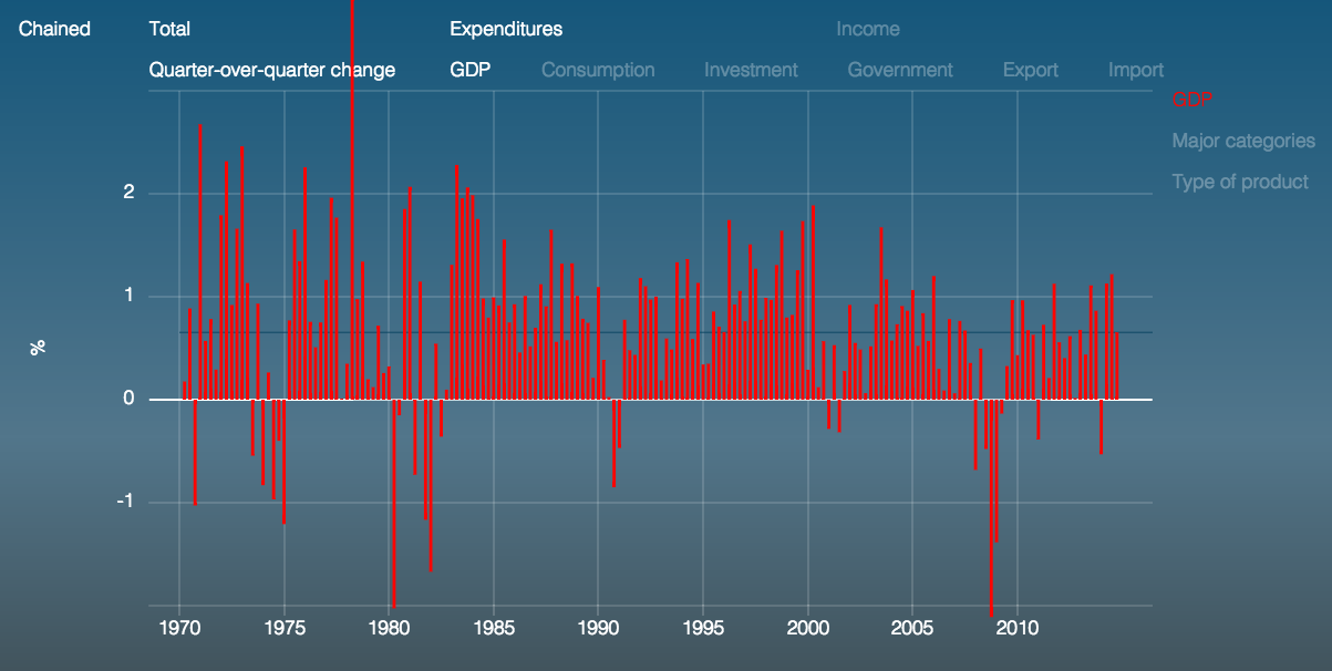
(hellomatrix.com/GDP.030)
Suppose we would like to forecast future GDP growth.
How can we develop a mathematical model of expected future growth rates that is consistent with the statistical properties of historical GDP?
First of all, we need to decide how we want to think about persistence of information over time.
For example, suppose this is the beginning of 2015, and we have three completely unrelated pieces of information, A, B and C, and A only affects GDP growth in the second quarter of 2015, and then A will become irrelevant, and B only affects the growth rate in the third quarter, and if we want to forecast the growth rate in fourth quarter we only need to know C, but none of this information will have any value for 2016.
Such a forecast model is theoretically possible but probably not very reasonable, and it probably makes more sense that our information about the state of the economy in Q3 of 2015 will not only be relevant for that one specific quarter but it will instead affect multiple consecutive time periods, and if that is true, GDP growth must have some persistent component and a successful forecast will identify this persistent component.
And, similar to forecasting the weather where our forecast for tomorrow is more accurate than the forecast for the day after tomorrow, and our best forecast for the same date next year is probably just the long-term average temperature for that season of the year, our beliefs about GDP growth might deviate from the long-run mean in the short term, but they should revert back to this mean in the long run.
In the following, I discuss a simple mathematical model that will allow us to analyze how much of the variation of future GDP we can possibly forecast and how persistent this forecast can be so that the model is consistent with the variation of growth rates and their timeseries correlation in the data.
And the goal of building this model is not to find the best possible statistical method to forecast GDP, but I am using GDP just as an example, and the real purpose of this analysis is to find a tractable model for expected growth rates that we can use for a discounted cash flow analysis as in Discounting Cash Flows.
Defining Growth Rates
Suppose we have a process \(Y_t,Y_{t+1},\dots\), such as quarterly GDP values, and define its growth rate as
$$
G_{t+1} = \frac{Y_{t+1}}{Y_t}
$$
This is a gross growth rate, so that \(G_{t+1}=1.05\) means that GDP grows by 5% from quarter \(t\) to \(t+1\).
Also, GDP growth is actually slightly more confusing since it is reported annualized, but we ignore annualization here and work with the actual growth rate and if we really wanted to annualize this, we would simply calculate \(G_{t+1}^4\).
Linear Growth
So we have a growth rate \(G\) and now suppose we would like to decompose this rate into its components such as, for example, expected growth rate and unexpected growth rate.
Here is a simple linear decomposition:
$$
G_{t+1} = \mu + \epsilon_{t+1}
$$
where we set \(E[\epsilon]=0\) so that \(\mu\) is the unconditional expectation of \(G\):
$$
E[G_{t+1}] = \mu
$$
Now that we have a one-period growth rate, we can examine how GDP grows over multiple periods by defining the compound growth rate from time \(t\) to \(t+\tau\) as
$$
G_t^{t+\tau} = G_{t+1}\times G_{t+2}\times\cdots\times G_{t+\tau}
$$
For example, the total growth over the next two quarters is
\begin{eqnarray}
G_t^{t+2} &=& (\mu+\epsilon_{t+1}) (\mu+\epsilon_{t+2})\\
&=& \mu^2 + \mu\epsilon_{t+1} + \mu\epsilon_{t+2} + \epsilon_{t+1}\epsilon_{t+2}
\end{eqnarray}
This last expression is a bit messy, even though maybe still somewhat tolerable, but we will run into problems once we try to calculate growth over more than two periods and if we extend this simple model to incorporate conditional expectations of near-term growth rates we will end up with a huge mess.
Therefore we now abandon this linear model in favor of a multiplicative model which will be much easier to work with.
Log-linear Growth
How can we decompose growth rates so that the multiperiod case remains tractable?
Since long-term growth is a product of short-term growth rates, we should decompose the short-term rates with products instead of sums.
We write our product as:
$$
G_{t+1} = e^{\mu+\epsilon_{t+1}},\hspace{1.5cm}E[\epsilon_t]=0,\hspace{0.5cm}\text{Var}[\epsilon]=\sigma_\epsilon^2
$$
And then the \(\tau\) period compound growth rate is simply given by
$$
G_t^{t+\tau} = e^{\mu+\epsilon_{t+1}}e^{\mu+\epsilon_{t+2}}\cdots e^{\mu+\epsilon_{t+\tau}}= e^{\tau\mu+\sum_{j=1}^\tau\epsilon_{t+j}}
$$
We can think of \(\mu+\epsilon\) as an approximate "net" growth rate, for example \(e^{0.05}\) = 1.0512 (and this approximation works well for numbers close to zero since we have as a linear approximation \(\log(1+x)\approx \log(1)+\log'(1)x = x\) ).
For convenience we typically write express the growth rate in linear form by taking logs:
$$
\hat G_{t+1} = \mu+\epsilon_{t+1},\hspace{1cm}\hat{G}_t^{t+\tau} = \tau\mu+\sum_{j=1}^\tau\epsilon_{t+j}
$$
where I use the notation \(\hat{X} = \text{log}(X)\).
For this simple model of growth rates we assume that the residuals \(\epsilon\) are pure noise and that they are independent and identically distributed or iid which means that they all come from the same distribution and are independent over time.
Since \(\epsilon\) are pure noise, the expected log growth rate is given by
$$
E[\hat G_t] = \mu
$$
This expectation of the log growth rate is interesting, but how can we calculate the expected growth rate \(E[G_t]\)?
It depends.
In general, we can always simulate a large number of realizations of \(G_t\) and then use the average simulated value as an estimator for the mean.
But there is one special case where we calculate the mean analytically, without resorting to a simulation, and that special case is the normal distribution.
If the log of a random variable \(Z\) is normally distributed then we say \(Z\) has a log-normal distribution and in this case we have:
$$
\log Z \sim \text{normal} \hspace{1cm}\implies\hspace{1cm} \log E[Z] = E[\log Z] + \frac{1}{2}\text{Var}[\log Z]
$$
So if we assume that the residuals \(\epsilon_t\) are normally distributed, then the log growth rate \(\hat{G}_t\) is normally distributed and therefore
$$
E[G_t] = e^{\mu+\frac{1}{2}\sigma^2}
$$
State Variable
Suppose on average log GDP grows at 1% per quarter but after conduction a sophisticated analysis of the current state of the economy, we come to the conclusion that GPD will grow at 1.5% for the next few quarters.
How do we incorporate the state of the economy into our model of growth rates?
We use a state variable.
Lets call our state variable \(X\) and write
$$
\hat G_{t+1} = \mu + X_t + \epsilon_{t+1}
$$
For example, if the unconditional average is 1% and we expect GDP to grow next quarter at 1.5%, then the state variable \(X_t\) is 0.5%.
We endow \(X\) with the subscript \(t\) since \(X_t\) represents the part of future GDP growth that is driven by the current state of the economy, and this notation also indicates that the value \(X_t\) is known at time \(t\).
Hence the expectation conditional on time \(t\) information is given by
$$
E_t[\hat G_{t+1}] = \mu + X_t
$$
Now if we believe that GDP growth next quarter will be unusually high, that probably does not imply that we believe GDP will continue to grow at an unusually high rate for all eternity. Therefore, and since we don't know much about the distant future, we need to build into our model some way for our near-term forecast to revert back to the mean in the long run.
We can write a simple mean-reverting process as
$$
X_{t+1} = \alpha X_{t} + \epsilon_{Xt+1}
$$
where
$$
0\le\alpha < 1,\hspace{0.5cm} \epsilon_{Xt}\sim\text{iid},\hspace{0.5cm} E[\epsilon_{Xt}]=0,\hspace{0.5cm}\text{Var}[\epsilon_{Xt}]=\sigma_{\epsilon X}^2
$$
and the parameter \(\alpha\) detemines how fast our current information becomes irrelevant and our conditional expectation of the growth rate \(G\) reverts to the unconditional mean \(\mu\).
This process is also called autoregressive process (of order 1) or AR(1)-process.
To keep the model simple, we also assume that the state variable residuals \(\epsilon_{Xt}\) are pure noise and they are independent of the growth rate residuals \(\epsilon_t\).
Since our state variable process works for every time \(t\), we have for example
$$
X_{t+2} = \alpha X_{t+1} + \epsilon_{Xt+2} = \alpha \Big(\alpha X_t + \epsilon_{Xt+1}\Big) + \epsilon_{Xt+2}
= \alpha^2 X_t + \alpha \epsilon_{Xt+1} + \epsilon_{Xt+2}
$$
and accordingly
$$
X_{t+\tau} = \alpha^\tau X_t + \sum_{j=1}^\tau\alpha^{\tau-j}\epsilon_{Xt+j}
$$
and therefore
\begin{eqnarray}
E_t[X_{t+\tau}] &=& \mu+\alpha^\tau X_t\\
\text{Var}_t[X_{t+\tau}] &=& \sum_{j=1}^\tau\alpha^{\tau-j}\sigma_{\epsilon X}^2
= \frac{\alpha(1-\alpha^\tau)}{1-\alpha} \sigma_{\epsilon X}^2
\end{eqnarray}
If we continue to solve the state variable process forward (or backward), we get in the limit
$$
X_t=\sum_{j=0}^\infty\alpha^j\epsilon_{t-j}
$$
So we get the unconditional variance:
$$
\text{Var}[X_t] = \frac{\sigma_{\epsilon X}^2}{1-\alpha^2}
$$
Hence we have for the total unconditional variance of the growth rate:
$$
\text{Var}[\hat G_{t+1}] = \text{Var}[X_t] + \text{Var}[\epsilon_{t+1}] = \frac{\sigma_{\epsilon X}^2}{1-\alpha^2} + \sigma_\epsilon^2
$$
For example, if \(\alpha\) is close to one, the growth rate \(G_t\) is almost a random walk and therefore the unconditional variance of this growth rate is large.
If we divide the variance of the state variable by the total variance, we get the proportion of (next-periods) variation that we can forecast with our current information:
$$
\frac{\text{Var}[X_t]}{\text{Var}[\hat G_{t+1}]} = \frac{\frac{\sigma_{\epsilon X}^2}{1-\alpha^2}}{\frac{\sigma_{\epsilon X}^2}{1-\alpha^2}+\sigma_\epsilon^2}
$$
Half-life of Information
The shock \(\epsilon_t\)affects \(X_{t+\tau}\) with factor \(\alpha^\tau\).
We define the half-life of the shock as
$$
\alpha^j = \frac{1}{2} \hspace{0.5cm}\Longleftrightarrow\hspace{0.5cm} j = \frac{\log 1/2}{\log\alpha}
$$
Here are the half-lives in number of periods for various \(\alpha\)s:
| \(\alpha\) | 0.1 | 0.2 | 0.3 | 0.4 | 0.5 | 0.6 | 0.7 | 0.8 | 0.9 | 0.95 |
| half-life | 0.30 | 0.43 | 0.58 | 0.76 | 1.00 | 1.36 | 1.94 | 3.11 | 6.58 | 13.51 |
Autocorrelation
Since the state variable is persistent, growth rates are correlated over time.
To calculate this correlation, we start with the covariance
\begin{eqnarray}
\text{Cov}[\hat G_t,\hat G_{t+\tau}] &=& \text{Cov}\Big[\mu+X_{t-1}+\epsilon_t, \mu+X_{t+\tau-1}+\epsilon_{t+\tau}\Big]\\
&=& \text{Cov}\Big[X_{t-1},\alpha^{\tau}X_{t-1}\Big]\\
&=& \alpha^\tau \frac{\sigma_{\epsilon X}^2}{1-\alpha^2}
\end{eqnarray}
and then we divide this expression by the product of the standard deviations to get the correlation
$$
\text{Corr}[G_t,G_{t+\tau}] = \alpha^\tau \frac{\frac{\sigma_{\epsilon X}^2}{1-\alpha^2}}{\frac{\sigma_{\epsilon X}^2}{1-\alpha^2}+\sigma_\epsilon^2}
$$
This correlation is also called autocorrelation or serial correlation.
The last equation tells us that our growth rate is strongly correlated over time if the state variable process is persistent and if a large proportion of the total variance is due to variations of the state variable.
Hence, unless growth rates are highly correlated over time, it is not possible to forecast a significant part of the growth rates far in the future.
For example, the quarterly autocorrelation of U.S. GDP is 0.38 (1947-2014), so if we assume information has a half-life of two quarters (\(\alpha=0.7\)) then we can predict about 0.38/0.7 = 54% of the variation of next quarters GDP.
Compound Growth
Compound growth rate:
$$
\hat G_t^{t+\tau} = \sum_{j=1}^\tau\hat G_{t+j} = \tau\mu+\sum_{j=1}^\tau X_{t+j-1} + \sum_{j=1}^\tau\epsilon_{t+j}
$$
Hence we need to know the compound state variable to calculate compound growth.
Lets start with the case of three periods:
\begin{eqnarray}
\sum_{j=0}^3 X_{t+j} &=& X_t + \Big(\alpha X_t+\epsilon_{Xt+1}\Big) + \Big(\alpha^2 X_t+\epsilon_{Xt+2}+\alpha\epsilon_{Xt+1}\Big) + \Big(\alpha^3 X_t+\epsilon_{Xt+3}+\alpha\epsilon_{Xt+2}+\alpha^2\epsilon_{Xt+1}\Big)\\
&=& X_t\sum_{j=0}^3\alpha^j + \Big(1+\alpha+\alpha^2\Big)\epsilon_{Xt+1} + \Big(1+\alpha\Big)\epsilon_{Xt+2} + \epsilon_{Xt+3}
\end{eqnarray}
So the general case is given by:
\begin{eqnarray}
\sum_{j=0}^\tau X_{t+j}
&=& X_t\sum_{j=0}^\tau\alpha^j + \sum_{j=1}^\tau\epsilon_{Xt+j}\sum_{i=0}^{\tau-j}\alpha^i
= \frac{1-\alpha^{\tau+1}}{1-\alpha}X_t + \sum_{j=1}^\tau\frac{1-\alpha^{\tau-j+1}}{1-\alpha}\epsilon_{Xt+j}
\end{eqnarray}
Plugging this back into the compound growth rate:
$$
\hat G_t^{t+\tau} = \tau\mu + \frac{1-\alpha^\tau}{1-\alpha}X_t + \sum_{j=1}^\tau\left(\frac{1-\alpha^{\tau-j}}{1-\alpha}\epsilon_{Xt+j} + \epsilon_{t+j}\right)
$$
Variance:
$$
\text{Var}\left[\hat G_t^{t+\tau}\right] = \tau\sigma_\epsilon^2+\sum_{j=1}^\tau\left(\frac{1-\alpha^{\tau-j}}{1-\alpha}\right)^2\sigma_{\epsilon X}^2
$$
Closed-form solution for the geometric series on the right hand side:
$$
\sum_{j=1}^\tau(1-\alpha^{\tau-j})^2 = \tau - 2\frac{\alpha(1-\alpha^\tau)}{1-\alpha} + \frac{\alpha^2(1-\alpha^{2\tau})}{1-\alpha^2}
$$
So we have for the conditional expectation:
$$
\log E_t[G_t^{t+\tau}] = \tau\mu + \alpha^\tau X_t + \frac{1}{2}\tau\sigma_\epsilon^2 + \frac{1}{2(1-\alpha)^2}\left(\tau - 2\frac{\alpha(1-\alpha^\tau)}{1-\alpha} + \frac{\alpha^2(1-\alpha^{2\tau})}{1-\alpha^2}\right) \sigma_{\epsilon X}^2
$$